机器学习笔记一:梯度下降算法
梯度下降算法
介绍
在数学中,梯度下降(通常也称为最速下降)是一种一阶迭代优化算法,用于寻找可微函数的局部最小值。 思路是在函数当前点的梯度(或近似梯度)的反方向重复走几步,因为这是最速下降的方向。 相反,沿梯度方向步进将导致该函数的局部最大值; 这个过程被称为梯度上升。
梯度下降法一般归因于奥古斯丁-路易斯柯西,他于1847年首先提出它。雅克阿达玛在1907年独立提出了类似的方法。它对非线性优化问题的收敛性质首先由Haskell Curry于1944年研究,用该方法 在接下来的几十年中得到越来越多的研究和使用。
基本原理
梯度下降方法基于以下的观察:如果实值函数\({F(\vec{x})}\)在点\({\vec{a}}\)可微且有定义,那么函数\({F(\vec{x})}\)在\({\vec{a}}\)点沿着梯度相反的方向\({-\nabla{F(\vec{a})}}\)下降最多。
因而,如果 \[{\mathbf {b}}={\mathbf {a}}-\gamma \nabla F({\mathbf {a}})\] 对于一个足够小数值\({\gamma>0}\)时成立,那么\({F({\mathbf {a}})\geq F({\mathbf {b}})}\)。
考虑到这一点,我们可以从函数F的局部极小值的初始估计\(x_0\)出发,并考虑如下序列 $,,,$,使得
\[\mathbf{x_{n+1}}=\mathbf{x_n}-\gamma_n \nabla F(\mathbf{x_n}),\ n \ge 0。\]
因此可得到 \[F(\mathbf{x_0})\geq F(\mathbf{x_1})\geq F(\mathbf{x_2})\geq \cdots \] 如果顺利的话序列\((\mathbf{x_n})\)收敛到期望的局部极小值。注意每次迭代步长\(\gamma\)可以改变。
举例:用梯度下降法求解\(\sqrt[4]{9}\)
理论分析
令\(x =
\sqrt[4]{9}\),问题即转化求解\(f(x) =
x^{4} -9\)的零点
由于开方运算得到的值具有非负性,因此只需讨论\(x>0\)的情况即可。
定义损失函数:
\[ L(x) = \frac{1}{2}(f(x)-0)^2 \]
对L(x)求导,得: \[ \frac{dL}{dx} = 4x^3 (x^4
- 9) \]
代码实现
1 | def f(x):#定义函数 |
探索学习率\(\alpha\)以及迭代初始值对结果的影响
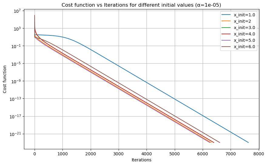
探索迭代初始值对结果的影响(控制迭代次数为20000,学习率为\(\alpha=10^{-5}\))
1 | import numpy as np |
探索最适合的迭代初始值(固定\(\alpha=10^{-5}\),迭代次数为20000)
1 | import numpy as np |
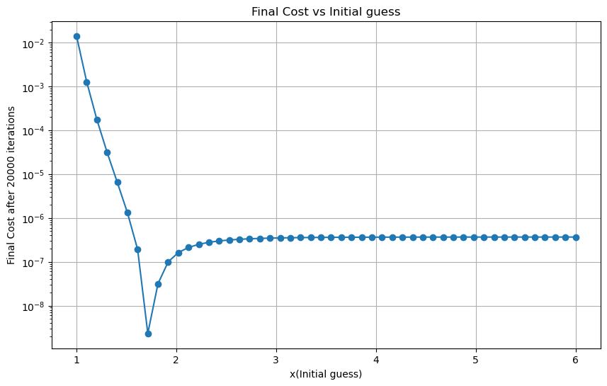
最好的迭代初始值: 1.7142857142857144
结论
对先减小再增大的定性分析:
越接近9的四次方根收敛得将会越快,越远离,收敛得越慢。
显然,当迭代初始值越接近9的四次方根,迭代的效果越好
探索\(\alpha\)对结果的影响(控制迭代次数为20000,迭代初始值为5.00)
选择迭代初始值为5的原因是:上面画图可得,3-5收敛速度比较平稳,不快不慢,容易体现\(\alpha\)的作用。 1
2
3
4
5
6
7
8
9
10
11
12
13
14
15
16
17
18
19
20
21
22
23
24
25
26
27
28
29
30
31
32
33
34
35
36
37
38
39
40
41
42
43
44
45
46
47
48
49import numpy as np
import matplotlib.pyplot as plt
# 定义函数
def f(x):
return x**4 - 9
# 定义损失函数
def L(x):
return 0.5 * (f(x)**2)
# 定义导数(梯度)
def slope_L(x):
return 4 * (x**3) * (x**4 - 9)
# 梯度下降法
def GD(alpha, x_init, max_times):
x = x_init
costs = []
for i in range(max_times):
cost = L(x)
costs.append(cost)
x = x - slope_L(x) * alpha
# 如果损失函数变化很小,提前终止迭代
#if len(costs) > 1 and np.abs(costs[-1] - costs[-2]) < 1e-15:
#break
if np.abs(costs[i]) < 1e-23:
break
return x, costs
# 绘制学习曲线
def plot_learning_process(alphas, x_init, max_times):
plt.figure(figsize=(10, 6))
for alpha in alphas:
x, costs = GD(alpha, x_init, max_times)
plt.plot(costs, label=f'α={alpha}')
plt.yscale('log')
plt.xlabel('Iterations')
plt.ylabel('Cost function')
plt.title('Cost function vs Iterations for different α values')
plt.legend()
plt.grid(True)
plt.show()
# 测试不同的 α
alphas = [10**(-5),10**(-6),10**(-7),10**(-4.5),10**(-4.49)]
plot_learning_process(alphas, 5, 20000)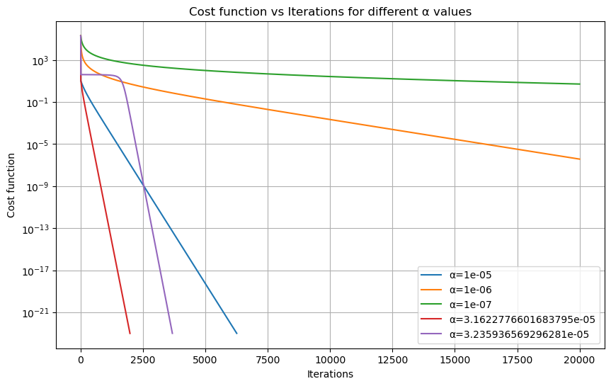
进行网格搜索,探索最适合的\(\alpha\)(固定迭代初始值为5,20000次迭代)
1 | import numpy as np |
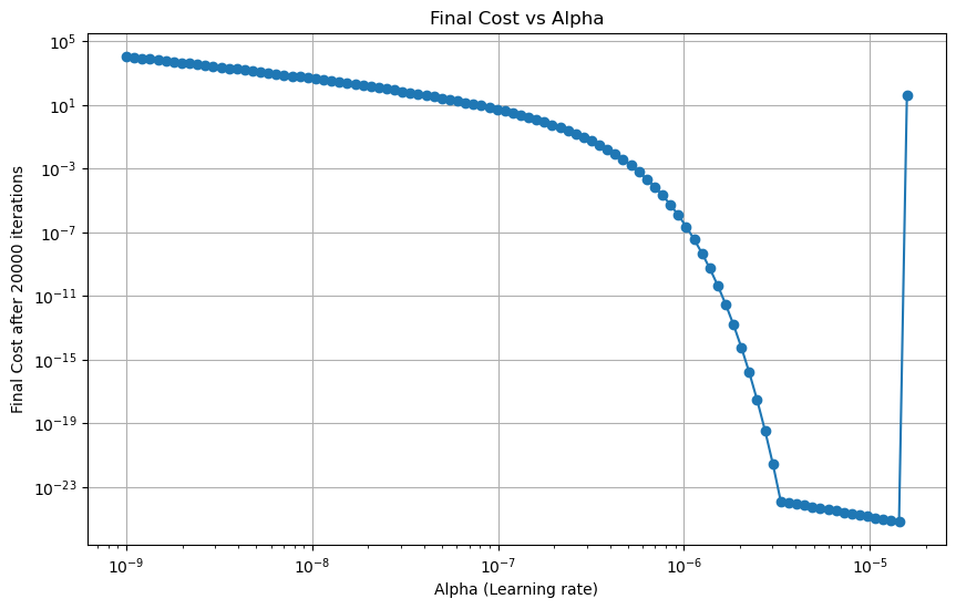
最好的alpha: 1.4373937679631066e-05
结论
先减小后增大的原因:
\(\alpha\)是学习步长,我们的优化空间是一个凹凸不平的面。如果步长太大,就永远走不到合适的坑里,会在山峰间跳来跳去,直到发散;如果步长太小,收敛则会太慢。
最好的\(\alpha\)在\(1.43*10^{-5}\)左右。
利用 python 库 scipy.optimize 探索其它优化方法(可选)。除了梯度下降方法,还有 BFGS等方法,尝试了解并使用它们。
BFGS算法
引用自维基百科BFGS算法
简介
在数值优化中,Broyden–Fletcher–Goldfarb–Shanno (BFGS) 算法是一种求解无约束非线性优化问题的迭代算法。和相关的Davidon–Fletcher–Powell算法类似,BFGS算法通过利用曲率信息对梯度进行预处理来确定下降方向。曲率信息则是通过维护一个使用广义的割线法逐步近似的关于损失函数的Hessian矩阵来获得。
算法
从起始点 \(x_0\) 和初始的 Hessian 矩阵 \(B_0\),重复以下步骤,\(x_k\) 会收敛到优化问题的解:
- 通过求解方程 \(B_k p_k = -\nabla f(x_k)\),获得下降方向 \(p_k\)。
- 在 \(p_k\) 方向上进行一维的优化(线搜索),找到合适的步长 \(\alpha_k\)。如果这个搜索是完全的,则 \[ \alpha_k = \arg\min f(x_k + \alpha p_k) \] 在实际应用中,不完全的搜索一般就足够了,此时只要求 \(\alpha_k\) 满足 Wolfe 条件。
- 令 \(s_k = \alpha_k p_k\),并且令 \(x_{k+1} = x_k + s_k\)。
- \(y_k = \nabla f(x_{k+1}) - \nabla f(x_k)\)。
- \(B_{k+1} = B_k + \frac{y_k y_k^T}{y_k^T s_k} - \frac{B_k s_k s_k^T B_k^T}{s_k^T B_k s_k}\)
函数 \(f(x)\) 表示要最小化的目标函数。可以通过检查梯度的范数 \(||\nabla f(x_k)||\) 来判断收敛性。如果 \(B_0\) 初始化为 \(B_0 = I\),第一步将等效于梯度下降,接下来的步骤会受到近似 Hessian 矩阵 \(B_k\) 的调节。
scipy.optimize代码实现
1 | import numpy as np |
最小值对应的 x: [1.73205081]
最小值: 1.9635447486648619e-19
参考资料
[1]菜鸟编程 python 教程 https://www.runoob.com/python/python-tutorial.html
[2]菜鸟教程-numpy教程 https://www.runoob.com/numpy/numpy-tutorial.html
[3]菜鸟教程-matplotlib教程 https://www.runoob.com/matplotlib/matplotlib-tutorial.html
[4]BFGS算法 https://zh.wikipedia.org/wiki/BFGS%E7%AE%97%E6%B3%95